Multiple Linear Regression model is used to develop a predictive model when there are multiple predictor/input variables. There are different approaches to find the best set of variables to select the best model like forward selection, backward selection and mixed selection method (combining both the methods) etc. The total number of possible models that can be made is given by the function below:
f(n) = C(n,1) + C(n,2) + C(n,3) + …..… + C(n,n)
This function is a step-wise variable selector for all the possible combinations where n = Number of input variables and n > 1
So for n=1,2,3 total number of possible models is 1,2,7 respectively.
R Function for model selection
As n increases, it becomes very lengthy to make so many models manually in R. That’s why it is better to use ‘ols_step_all_possible()’ function which is available in the package called ‘olsrr’. The interesting thing about this function is that it returns a data frame which gives the result for each of the models along with the respective variables taken and different parameters like R square (rsquare), Adjusted R square (adjr), Predicted R square (predrsq), Akaike Information Criteria (AIC) and many more.
Steps for Selecting the Best Model
While selecting the best model we look for maximum Adjusted R square (or both R square and Adjusted R square) and minimum AIC value. There are other parameters which we can also see are Final Prediction Error (FPE), Sawa’s Bayesian Information Criteria (SBC), Scharwz Bayesian Criteria (SBIC), Estimated Error of Prediction (MSEP) (Assuming multivariate normality), Amemiya Prediction Criteria (APC).
mtcars is an inbuilt dataset available in R on car with many variables. We are going to use this dataset to demonstrate and explain the steps and codes. Here we are selecting 4 variables “cyl”, “disp”, “hp”,”drat” as inputs and “mpg” as output variable.
Sample code:
df <- mtcars[, c(“mpg”, “cyl”, “disp”, “hp”,”drat”)]
lin_mod_1 <- lm(mpg ~ ., data = df) # Linear Regression Model
install.packages(“olsrr”) # Install the required package.
library(olsrr) # Load the library
k <- ols_step_all_possible(lin_mod_1)
write.csv(k, “results.csv”, row.names = FALSE) # Save the data frame as csv
plot(k)
Interpretation:
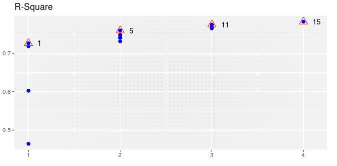
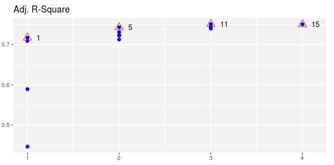
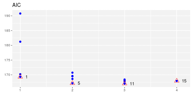
Out of the 4 models marked having the highest adjr, the two best models to select is mindex 11 and 15 with three and four variables respectively. Comparing these two models, we see that the one with variables disp, hp, drat has slightly higher adjr and has lower AIC, predrsq and fpe than the four-variable model. So the model having the predictors disp, hp and drat is the best model.
We can also see the same result by plotting k. The x-axis shows the number of variables at a time and y-axis shows the parameter values.
Note: This function does not take care of multicollinearity in between the predictors. Also if there is any interaction effect, so we can also see that by creating new variables in the data and then running the function. If you want to learn more you can check out our Business Analytics course.


